Become a more efficient data analyst, a comprehensive guide to pandas

A short introduction to pandas

Photo by Sid Balachandran on Unsplash

You have a large dataset with some compelling insights, but you are still far away to figure out how to extract those insights or have a glimpse of statistics on the data. Pandas come in very handy in those situations.

Pandas quickly read and understand data and give you insights so you can be more efficient at your role. To get started with pandas, we need to get comfortable with two data structures in pandas Series and Data Frame. While they are not a universal solution for every problem, however, they provide a solid, easy-to-use basis foundation for most applications.

Series — 1-D array-like object.

Data Frame — A tabular data structure in pandas just like in excel.

Start with importing the package:

import pandas as pd

The most popular convention to import pandas is with the pd alias.

Series

Creating a series by passing a list of values, pandas will create a default integer index

data = pd.Series([1,2,3,4])

left one’s are indexes(0,1,2,3) and the right ones(1,2,3,4) are the values.

Check the values & index

data.values
data.index

Changing the default index values 0,1,2,3 to new custom index values

data1 = pd.Series([1,2,3,4], index = [‘a’, ‘b’, ‘c’, ‘d’]
data1

Data selection

Single value selection will select the value corresponding to the index value ‘a’.

data1[‘a’]

Data selection -multiple values

data1[[‘a’,’b’]]

DataFrame

A Dataframe is a tabular data-like structure just like excel. It contains an ordered collection of columns, that can be of different value types (numeric, string, boolean, etc.). It has both a row and column index.

Creating a DataFrame

DataFrame will have its index assigned as Series.

Below we create a data frame with countries name, year, and population in a particular year in millions.

data = {‘Country’: [‘India’, ‘UK’, ‘USA’, ‘Japan’, ‘Ireland’],
‘year’: [2020, 2021, 2022, 2023, 2024],
‘population’: [1.4, 1.2, 0.5, 0.4, 1.6]}
df = pd.DataFrame(data)
df

You can specify the sequence of columns, output will exactly be the same as you pass it.

df1 = pd.DataFrame(data, columns = [‘population’,’year’,’Country’])
df1

Accessing Columns in a data frame

By Dict-type notation:

df1[‘Year’]

By dot notation:

df1.Country

Importing a CSV file

data = pd.read_csv(‘pokemon.csv’)

you can see the type of data and how much data ‘pokemon’ contain.

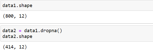
len only counts the number of rows, if you want to have a look at both the number of rows and columns we can do that with the .shape. In our data, we have 800 rows and 12 columns.

Display all columns and their data types with .info()

This provides the total number of index range, a number of columns in the data set, type of columns(count), and data type.

We can quickly analyze our dataset contains three different types of data types(integer, object, boolean).objects are the strings values.

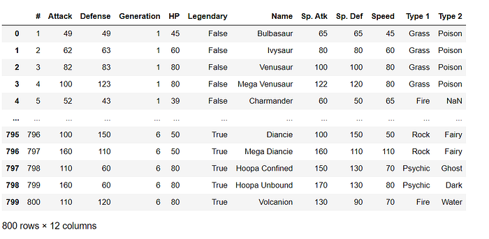
Top view

data.head()# by defalut it shows only 5 rows.
# data.head(n=10) # will display the 10 number of rows.

Bottom View

data.tail()

By default head and tail only shows only 5 rows. you can change this with pd.set_option if you have a data frame with hundred of columns. You can also specify how many columns you want to have a look at.

pd.set_option(“display.max.columns”, None) # will show all columns
pd.set_option(‘display.max_columns’, 50)# will show 50 columns
# will show top 50 rows
data.head(50)
# will show last 100 rows
data.tail(100)

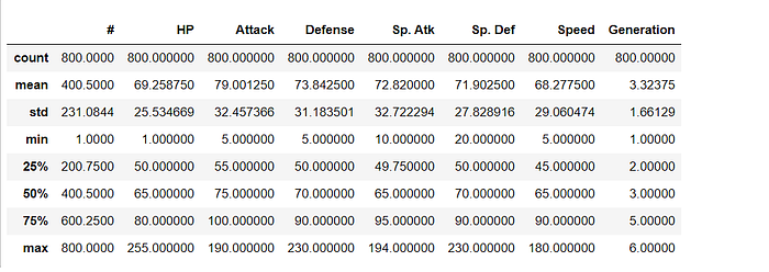
For a quick statistic, summary use describe()

This will provide descriptive statistics of all the numeric columns in the dataset.

data.describe()

Transpose the data

data.T

Sorting by axis

axis = 0 refers to rows, axis =1 to columns.

data.sort_index(axis=1, ascending=True)
# it sorts the columns alphabetically.

Sorting by value

data.sort_values(by=”Name”)

Change the column names into a data frame

data.rename(columns = { ‘Name’ : ‘Pokemon name’, ‘Type 1’: ‘ first type’})

Dropping the columns

data.drop(columns=[‘Pokemon name’,’first type', ‘Type 2’])

Rows subset observations

data[data.Length > 10] #Extract rows that meet logical criteria.
df.sample(frac=0.5) #Randomly select fraction of rows.
df.sample(n=10) #Randomly select n rows.
df.iloc[10:20] #Select rows by position.

Select rows and columns using labels(loc):

you can access rows and columns by their corresponding labels into a pandas data frame.

Select a single row by label:

this gives all the details for the first row.

data.loc[0]

Accessing multiple rows by label:

data.loc[[0,1]] # selecting the rows at index 0 and 1

Accessing by row and column:

data.loc[0,”Type 2"] # selection of index 0 and colum namne Type 2

Selecting Single row, multiple columns:

data.loc[1,[‘Name’,’Attack’,’Defense’]]

Select by index position(iloc):

Row by index location:

data.iloc[1] # index starts from zero

Column by index location:

data.iloc[:, 3] # ‘Type 2’ column in pokemon data

Slicing rows and columns using labels:

Slice rows by labels

selecting the rows at locations 1–3 and all the columns.

data.loc[1:3, :]

Slice columns of labels

selecting at locations 1–3 and only two column values.

data.loc[1:3, ‘Type 1’:’Type 2']

Slice rows and columns using position(iloc):

Index starts from 0 to (number of rows/columns -1).

slice rows by index position

data.iloc[0:3,:]

slicing columns by index position

data.iloc[:,1:3]

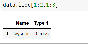
slice row and columns by index position

data.iloc[1:2,1:3]

Handling missing values

In pandas dropna() function is being used to remove rows and columns with Null/NaN values. This function used a lot when there is any missing data in the data frame.

The syntax of dropna() function looks as per the below.

dropna(self, axis=0, how=”any”, thresh=None, subset=None, inplace=False)

• axis: possible values are 0 or 1 default is 0. if 0 drop rows, if 1 drop columns.
• how: possible values are (any, all), default is any. If any drop the row/column where values are null. If all, drop row/columns.
• thresh: an int to specify the threshold for the drop.
• subset: specifies the rows/columns to look for null values.
• inplace: a boolean value. If True, the source DataFrame will be changed and it will return none.

Dropping all the rows with null values. After removing na we have 414 rows left in the data frame.

Dropping the columns with missing values

Merging datasets

Merge or join operations combine data sets by linking rows using one or more keys.

Main arguments of pd.merge and their description

left -> DataFrame to be merged on the left side.

right->DataFrame to be merged on the right side.

how ->One of ‘inner’, ‘outer’, ‘left’ or ‘right’. ‘inner’ by default

on ->Column names to join on. Must be found in both DataFrame objects. If not specified and no other join keys given, will use the intersection of the column names in left and right as the join keys.

we create two data frames to go through with all of these merge operations in a data frame.

First data frame

Second Data frame

Inner Join

join matching rows from df2 to df1

returns a data frame containing all the rows of the left data frame.

pd.merge(df1, df2,how=’left’, on=’key’)

right join -

join matching rows from df1 to df2

all the rows of the right data frame are taken as it is and only those of the left data frame that are common in both.

pd.merge(df1, df2,how=’right’, on=’key’)

inner join

returns a data frame with only those rows that have common in both data frames.

pd.merge(df1, df2,how=’inner’, on=’key’)

outer join

retain all of the data that is available in all rows and all values

pd.merge(df1, df2,how=’outer’, on=’key’)

In conclusion, these are the most common pandas functions that help you dig around your data for further analysis.